(Partial) autocorrelation is used to detect autocorrelation in time series data, that is, the correlation between current and past observations. It can help determine the autocorrelation patterns of time series data, thereby selecting the appropriate time series model.

    Data description:

    Background description:

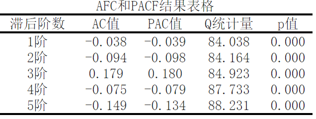
    Autocorrelation is used to measure the correlation between the current and previous observations in time series data. The AC value represents the correlation between the current observation value and the previous observation value of a specific lagging order, while the PAC value represents the correlation between the current observation value and the previous observation value of a specific lagging order by eliminating interference from other lagging orders. In this example, we conducted a (partial) autocorrelation test to evaluate the autocorrelation of time series data by calculating autocorrelation coefficients (AC values) and partial autocorrelation coefficients (PAC values) with lag orders of 1 to 5, as well as corresponding Q-statistics and p-values.

    The analysis results are as follows:

    In this example, we can observe the following aspects:

    Positive and negative values of AC and PAC: The positive and negative values of AC and PAC can tell us about the positive or negative correlation in time series data. A negative value indicates a negative correlation, meaning that when the current observation value is large, the previous observation value is small; A positive value indicates a positive correlation, and when the current observation value is large, the previous observation value is also large.

    Q-statistic and p-value: Q-statistic is a statistic that tests the correlation between observed values and lagged observations, assuming that time series data does not have autocorrelation. The p-value represents the probability of a significant correlation between observed values and lagged observations under given assumptions. Here, the p-values are all 0.000，说明观测值与滞后观测值之间存在显著的相关性。

    Autocorrelation Function (AFC) is a graph that describes the autocorrelation of time series data. This figure shows the change in AC value corresponding to the lagging order. According to the given order of lag, the closer the AC value is to 1, the stronger the correlation between the current observation value and the lag observation value.

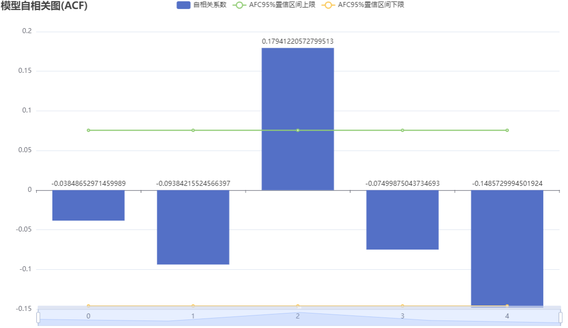
    The above figure shows the autocorrelation graph (ACF), including coefficients, upper confidence limits, and lower confidence limits. The horizontal axis represents the number of delays, and the vertical axis represents the autocorrelation coefficient. The autocorrelation (ACF) graph is truncated in the q order, while the partial autocorrelation (PACF) graph is trailing. The ARMA model can be simplified to the MA (q) model. If both autocorrelation and partial autocorrelation graphs are trailing, the most significant order (minimum value) in PACF and ACF graphs can be combined as the p and q values.

    If both autocorrelation and partial autocorrelation graphs are truncated, it is possible to choose to replace them with a higher difference or not suitable for establishing an ARMA model. Truncation is within the confidence interval, where ACF or PACF remains constant to zero (or fluctuates randomly around 0) after a certain order. Trailing refers to the fact that within the confidence interval, ACF or PACF always has a non-zero value and does not appear to be equal to zero after a certain order (or fluctuate randomly around 0).

    The Partial Autocorrelation Function (PACF) is used to evaluate the correlation between the current observations and the previous observations of a specific lag order. The PACF diagram shows the variation of PAC values corresponding to the order of hysteresis. Unlike AFC plots, PACF plots observe the correlation after eliminating interference from other lagging orders.

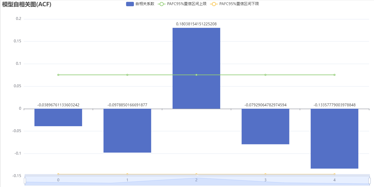
    The above figure shows a partial autocorrelation graph (PACF), including coefficients, upper and lower confidence limits. The partial autocorrelation (PACF) graph is truncated at the p-th order, while the autocorrelation (ACF) graph is trailing. The ARMA model can be simplified to the AR (p) model. If both autocorrelation and partial autocorrelation graphs are trailing, the most significant order (minimum value) in PACF and ACF graphs can be combined as the p and q values.

    If both autocorrelation and partial autocorrelation graphs are truncated, it is possible to choose to replace them with a higher difference or not suitable for establishing an ARMA model. Truncation is within the confidence interval, where ACF or PACF remains constant to zero (or fluctuates randomly around 0) after a certain order. Trailing refers to the fact that within the confidence interval, ACF or PACF always has a non-zero value and does not appear to be equal to zero after a certain order (or fluctuate randomly around 0).

    Reference:

    [1]Box, G. E., Jenkins, G. M., Reinsel, G. C., & Ljung, G. M. (2015). Time series analysis: Forecasting and control (5th ed.). John Wiley & Sons.

    [2]Wei, W. W. S. (2006). Time series analysis: Univariate and multivariate methods. Pearson Education.

    [3]Lutkepohl, H. (2017). New introduction to multiple time series analysis. Springer.

    [4]Cryer, J. D., & Chan, K. S. (2008). Time series analysis: With applications in R (2nd ed.). Springer.[5]Hamilton, J. D. (1994). Time series analysis. Princeton University Press.  

关注微信公众号发送【示例数据】获取SPSSMAX练习示例数据。