Cubic curve regression analysis is also a regression analysis method used to study the relationship between two variables. In cubic curve regression analysis, we assume that there is a cubic equation relationship between two variables, and analyze the data to determine the coefficients of the cubic equation. Then, this cubic equation can be used to predict the value of one variable, given the value of another variable. Similar to quadratic curve regression analysis, cubic curve regression analysis is usually used to study the changing trends of natural phenomena or market trends. It should be noted that cubic curve regression analysis has a higher equation complexity compared to quadratic curve regression analysis, therefore requiring more data points to determine coefficients.

    Background description:

    In this study, we focused on the impact of the independent variable A1 on the dependent variable A2 and used a cubic curve regression method. These variables are data obtained through a survey questionnaire to evaluate participants' characteristics or behavior on a specific question. Cubic curve regression is a statistical analysis method used to establish a model with a cubic polynomial relationship between the independent and dependent variables. Compared to simple linear regression models, cubic curve regression models can more accurately describe the influence of independent variables on dependent variables, as they consider the effects of cubic and quadratic terms. Specifically, cubic curve regression will fit a cubic polynomial model to the data to minimize the error between the model and the actual observation points.

    The analysis results are as follows:

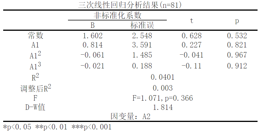
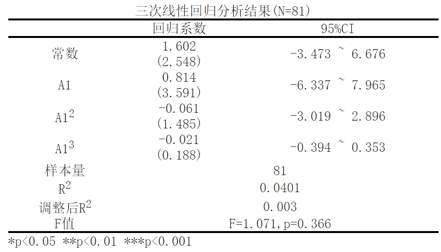
     From linear regression analysis, it can be seen that the model formula is A2=1.602+0.814 * A1-0.061 * A1, with A2 as the dependent variable and ['A1 '] and its square and cubic indicators as independent variables for cubic regression analysis. From the above table, it can be seen that the model formula is: A2=1.602+0.814 * A1-0.061 * A1_ Square -0.021 * A1_ Cube; The R-squared value of the model is 0.0401, which means that ['A1 '] and its squared and cubic indicators can explain the 4.01% change in A2. A2=1.602+0.814 * A1-0.061 * A1_ Square -0.021 * A1_ Cube

    Reference:

    [1]Golub, G. H., & Van Loan, C. F. (2013). Matrix computations (4th ed.). Johns Hopkins University Press.

    [2]Liu, X., Zhu, X., Li, Z., & Li, X. (2017). A simulation comparison of inverse distance weighting and cubic spline interpolation for DEM generation. Journal of Earth Science, 28(6), 1089-1096.

    [3]Fernández-Hernández, J., García-Sánchez, Á., & Moya-Gómez, B. (2015). Local forecasting methods based on regression models for time series modeling and prediction. Neurocomputing, 149(PB), 1224-1232

关注微信公众号发送【示例数据】获取SPSSMAX练习示例数据。