LSD post hoc test is named after Least Significant Difference and is also a common multiple comparison method. Similar to the Tukey post test, the LSD post test is also used to determine significant differences between two or more groups. Usually, in analysis of variance, if there is a hypothesis of homogeneity of variance, LSD post test is used.

    Data description:

    Background description:

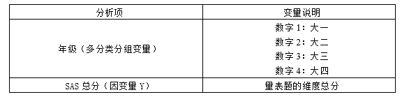
    This analysis of variance is conducted on the performance of students of different grades in multiple projects. We have four grades (1, 2, 3, and 4) and have evaluated the total SAS score among them.

    The purpose of variance analysis is to determine whether there are significant differences between different groups and further understand the degree of differences between different groups in each project. By comparing the mean, standard deviation, F-value, and p-value, we can determine the impact of groups on different projects and the comparison results between them.

    The purpose of variance analysis is to determine whether there are significant differences between different groups and further understand the degree of differences between different groups in each project. By comparing the mean, standard deviation, F-value, and p-value, we can determine the impact of groups on different projects and the comparison results between them.

    The analysis results are as follows:

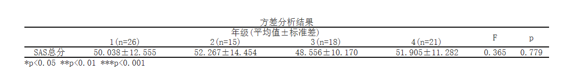
     From the above table, it can be seen that conducting one-way analysis of variance (also known as one-way analysis of variance) on the total SAS score showed a total average of 50.612, a total standard deviation of 11.976, an F-value of 0.365, and a p-value of 0.779, indicating that there was no significant difference in the total SAS scores among different groups (p>0.05).

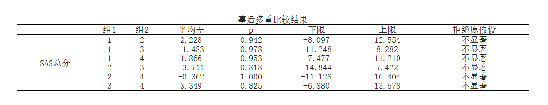
    From the comparison afterwards, it can be seen that,

    The results showed that there was no significant difference between item 3.0 and item 1.0 in the total SAS score of the variable. The average value of item 3.0 was 48.556, and the average value of item 1.0 was 50.038. The difference in the average value was -1.483, with a p-value of 0.680>0.05.

    The results showed that there was no significant difference between item 3.0 and item 4.0 in the total SAS score of the variable. The average value of item 3.0 was 48.556, and the average value of item 4.0 was 51.905. The difference in the average value was -3.349, with a p-value of 0.340>0.05.

    The results showed that there was no significant difference between item 3.0 and item 2.0 in the total SAS score of the variable. The average value of item 3.0 was 48.556, and the average value of item 2.0 was 52.267. The difference in the average value was -3.711, with a p-value of 0.394>0.05.

    The results showed that there was no significant difference between item 1.0 and item 4.0 in the total SAS score of the variable. The average value of item 1.0 was 50.038, and the average value of item 4.0 was 51.905. The difference in the average value was -1.866, with a p-value of 0.599>0.05.

    The results showed that there was no significant difference between item 1.0 and item 2.0 in the total SAS score of the variable. The average value of item 1.0 was 50.038, and the average value of item 2.0 was 52.267. The difference in the average value was -2.228, with a p-value of 0.607>0.05.

    The results showed that there was no significant difference between item 4.0 and item 2.0 in the total SAS score of the variable. The average value of item 4.0 was 51.905, and the average value of item 2.0 was 52.267. The difference in the average value was -0.362, with a p-value of 0.933>0.05.

    Reference:

    [1]Armstrong R A. When to use the Bonferroni correction[J]. Ophthalmic & Physiological Optics the Journal of the British College of Ophthalmic Opticians, 2015, 34(5):502-508.

    [2]张厚粲, 徐建平. 现代心理与教育统计学.第3版[M]. 北京师范大学出版社, 2009.

    [3]颜虹,徐勇勇. 医学统计学.第3版[M].人民卫生出版社,2017.

关注微信公众号发送【示例数据】获取SPSSMAX练习示例数据。